Difference between revisions of "Contrib:KeesWouters/shell/plotcoq3dparavis"
Keeswouters (Talk | contribs) m |
Keeswouters (Talk | contribs) m (→Reaction forces of the shell) |
||
| (132 intermediate revisions by the same user not shown) | |||
| Line 1: | Line 1: | ||
* [[Contrib:KeesWouters/shell]] | * [[Contrib:KeesWouters/shell]] | ||
| − | * [[Contrib:KeesWouters]] | + | * [[Contrib:KeesWouters]] |
| + | * [[http://www.caelinux.org/wiki/index.php/Contrib:KeesWouters/shell/plotcoq3d postprocessing by Salome postpro]] <br/><br/> | ||
=='''Post processing of COQUE-3D results by ParaVis'''== | =='''Post processing of COQUE-3D results by ParaVis'''== | ||
| − | |||
| − | This contribution is | + | |
| + | '''under construction''' | ||
| + | |||
| + | This contribution is valid for Code-Aster version 11.3 (August 2013) and later. | ||
In this contribution the main (and only) focus is on the postprocessing of the displacements and stresses of shell COQUE-3D elements. The centre nodes of tria7 and quad9 elements used for the discription of the displacements field of COQUE_3D poses some nasty problems in the postprocessing by ParaVis. To overcome this problem the results are projected on the original quadratic mesh without the centre node. Snapthrough of a slightly bend shell is used to visualise the displacements and von Mises stresses in ParaVis. The non linear command STAT_NON_LINE is used to step through the displacements at the centre line. | In this contribution the main (and only) focus is on the postprocessing of the displacements and stresses of shell COQUE-3D elements. The centre nodes of tria7 and quad9 elements used for the discription of the displacements field of COQUE_3D poses some nasty problems in the postprocessing by ParaVis. To overcome this problem the results are projected on the original quadratic mesh without the centre node. Snapthrough of a slightly bend shell is used to visualise the displacements and von Mises stresses in ParaVis. The non linear command STAT_NON_LINE is used to step through the displacements at the centre line. | ||
=='''Definition of the geometry'''== | =='''Definition of the geometry'''== | ||
| − | + | This time the geometry has been drawn in FreeCAD. It is good enough at this moment (agusut 2013) to draw a more or less complex geometry, although, in this case, it wouldnot have been much more effort to construct it in Salome. Anyway, I import the *.iges geometry from FreeCAD into Salome and mesh it there. The freeCAD dimensions are supposed to be in [mm] and the have been converted to [m] by Salome. Hence all dimensions are in [m] from here onwards. | |
| − | + | Noted that due to the partioning in Salome a double row of beams (seg3) elemenents is available at the centre line. | |
| − | + | * [[Image:kw_st_freecad2a.png]] | |
| + | |||
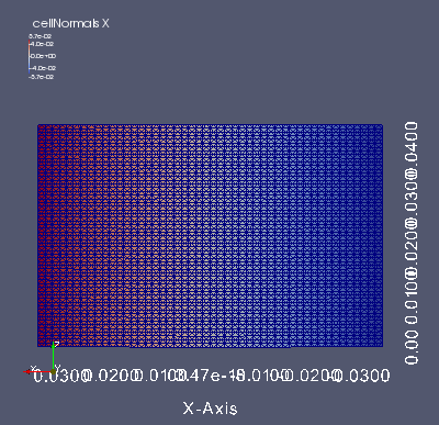
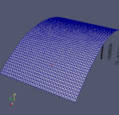
| + | A slightly bend shell is used to show snapthrough behaviour by Code-Aster. Main dimensions are Length x Width = [-0.035...0.035] x [0...0.045]. The maximum out-of-plane offset in y direction at the centre line is 0.001 (see right hand side figure below. Note that the offset has been scaled by a factor 10 and the y coordinate reflects this factor). The thickness is defined in the Code Aster *.comm file and can be changed any time: thickness th = 0.000125.<br/> | ||
| + | See below for some items regarding ParaVis. | ||
| + | |||
| + | * [[Image:kw_snapthrough_normalx2.png]] * [[Image:kw_snapthrough_normalx3.png]] | ||
| + | |||
| + | Units have to be consistent and will be: | ||
* length and displacments [m] | * length and displacments [m] | ||
* forces [N] and moments [Nm] and | * forces [N] and moments [Nm] and | ||
* Youngs' modulus and stresses [Pa] | * Youngs' modulus and stresses [Pa] | ||
| + | |||
'''Boundary conditions and loads:''' <br> | '''Boundary conditions and loads:''' <br> | ||
| − | * all | + | * all dofs are fixed on short side in negative x direction (Lxmin): |
** (DX=0.0, DY=0.0, DZ=0.0, DRX=0.0, DRY=0.0, DRZ=0.0) <br> | ** (DX=0.0, DY=0.0, DZ=0.0, DRX=0.0, DRY=0.0, DRZ=0.0) <br> | ||
| − | * | + | * all translational dofs are fixed on short side in positive x direction (Lxplus): |
| − | ** ( | + | ** (DX=0.0, DY=0.0, DZ=0.0) <br> |
| − | * | + | * load: prescribed displacement at centre line in y direction, out-out-of-plane, vertical (Lxcentre): |
| + | ** dy = 0.0...0.0014 [m]<br/> | ||
| + | |||
'''Material:'''<br/> | '''Material:'''<br/> | ||
Material steel<br/> | Material steel<br/> | ||
| Line 28: | Line 41: | ||
* Nu = 0.28 | * Nu = 0.28 | ||
* rho = 7850 kg/m3 (not needed) | * rho = 7850 kg/m3 (not needed) | ||
| − | |||
=='''A rough discription of the Code-Aster commands'''== | =='''A rough discription of the Code-Aster commands'''== | ||
| Line 50: | Line 62: | ||
#* print results of modified and initial model (results of the modified model are only printed to show that they are not fully what you expect) | #* print results of modified and initial model (results of the modified model are only printed to show that they are not fully what you expect) | ||
| − | Steps 1 to 8 are fairly standard and are | + | Steps 1 to 8 are fairly standard and only the commands are given here.<br/> |
| − | The stresses can be provided at the top, the centre and the bottom of the shell plane. These layers are denoted by 'SUP', 'MOY', and 'INF' in Code-Aster (superieur, moyenne et inferieur je pense) and depends on the normal vector of the shell elements (see step 3 in the general flow). These can be changed by the ORIENT command. In the next part all the commands could be given for the three layers, but it has been described here only for 'SUP' to keep it tidier. In the *.comm file at the end the complete command file can be downloaded with all layers excecuted. | + | The stresses can be provided at the top, the centre and the bottom of the shell plane. These layers are denoted by 'SUP', 'MOY', and 'INF' in Code-Aster (superieur, moyenne et inferieur je pense) and depends on the normal vector of the shell elements (see step 3 in the general flow). These can be changed by the ORIENT command. In the next part all the commands could be given for the three layers, but it has been described here only for 'SUP' to keep it tidier. In the *.comm file at the end the complete command file can be downloaded with all layers excecuted, see next chapter. |
| − | ==='''Short description of CALC_CHAMP, POST_CHAMP and PROJ_CHAMP''' | + | |
| + | # reading initial mesh | ||
| + | initMesh=LIRE_MAILLAGE(FORMAT='MED',INFO=1,); | ||
| + | |||
| + | #define shell (coque_3D) model; | ||
| + | # we have to add centre nodes with CREA_MAILLAGE | ||
| + | modiMesh=CREA_MAILLAGE(MAILLAGE=initMesh,INFO=1, | ||
| + | MODI_MAILLE=(_F(TOUT='OUI',OPTION='TRIA6_7',), | ||
| + | _F(TOUT='OUI',OPTION='QUAD8_9',),),); | ||
| + | |||
| + | modiMesh=MODI_MAILLAGE(reuse=modiMesh, | ||
| + | INFO=1, | ||
| + | MAILLAGE=modiMesh, | ||
| + | ORIE_NORM_COQUE=_F(GROUP_MA=('shell',), | ||
| + | VECT_NORM=(0.0,1.0,0.0), | ||
| + | NOEUD='N1'),); ## use ORIE_PEAU_2D if eg. z=0 for all nodes | ||
| + | |||
| + | iniModel=AFFE_MODELE(MAILLAGE=initMesh, | ||
| + | AFFE=_F(TOUT='OUI', | ||
| + | PHENOMENE='MECANIQUE', | ||
| + | MODELISATION='3D',),); | ||
| + | |||
| + | coqModel=AFFE_MODELE(MAILLAGE=modiMesh, | ||
| + | AFFE=_F(TOUT='OUI', | ||
| + | PHENOMENE='MECANIQUE', | ||
| + | MODELISATION='COQUE_3D',),); | ||
| + | |||
| + | th = 0.000125 | ||
| + | shellch=AFFE_CARA_ELEM(MODELE=coqModel,COQUE=_F(GROUP_MA='shell',EPAIS=th,),); | ||
| + | |||
| + | steel=DEFI_MATERIAU(ELAS=_F(E=2.100e11,NU=0.28,RHO=7850.0),); | ||
| + | material=AFFE_MATERIAU(MAILLAGE=modiMesh,AFFE=_F(TOUT='OUI',MATER=steel,),); | ||
| + | |||
| + | # define BC and loads | ||
| + | xp = 'Lxplus' | ||
| + | xm = 'Lxmin' | ||
| + | xc = 'Lxcentre' | ||
| + | |||
| + | hinghing=AFFE_CHAR_MECA(MODELE=coqModel, | ||
| + | DDL_IMPO=(_F(GROUP_MA=xp,DX=0.0,DY=0.0,DZ=0.0), | ||
| + | _F(GROUP_MA=xm,DX=0.0,DY=0.0,DZ=0.0),),); | ||
| + | |||
| + | fixhing=AFFE_CHAR_MECA(MODELE=coqModel, | ||
| + | DDL_IMPO=(_F(GROUP_MA=xp,DX=0.0,DY=0.0,DZ=0.0,DRX=0.0,DRY=0.0,DRZ=0.0), | ||
| + | _F(GROUP_MA=xm,DX=0.0,DY=0.0,DZ=0.0),),); | ||
| + | |||
| + | clamped = fixhing # or hinghing | ||
| + | |||
| + | ydispmax = -0.0020 | ||
| + | dispz=AFFE_CHAR_MECA(MODELE=coqModel, | ||
| + | DDL_IMPO=(_F(GROUP_MA=xc,DY=ydispmax),),); | ||
| + | |||
| + | # load stepping | ||
| + | # define 50, linearly increasing steps (time INST: 0.0 to 1.0, ramp 0.0 to 1.0) | ||
| + | tsteps = 50 | ||
| + | time=DEFI_LIST_REEL(DEBUT=0.0, | ||
| + | INTERVALLE=_F(JUSQU_A=1.0,NOMBRE=tsteps,), | ||
| + | INFO=2,TITRE='time',); | ||
| + | |||
| + | ramp=DEFI_FONCTION(NOM_PARA='INST', | ||
| + | VALE=(0.00,0.00, | ||
| + | 0.50,0.50, | ||
| + | 1.00,1.00,), | ||
| + | INFO=2,TITRE='ramp',); | ||
| + | |||
| + | # apply automatic time stepping, minimum step size 0.0005, maximum step size defined by '''ramp''' | ||
| + | deflist = DEFI_LIST_INST(DEFI_LIST=_F(METHODE ='AUTO', | ||
| + | LIST_INST = time, | ||
| + | PAS_MINI = 0.0005),); | ||
| + | |||
| + | # non linear static calculation, elastic behaviour, large displacement and rotations '''GROT_GDEP''' | ||
| + | RESU=STAT_NON_LINE(MODELE=coqModel, | ||
| + | CHAM_MATER=material, | ||
| + | CARA_ELEM=shellch, | ||
| + | EXCIT=(_F(CHARGE=clamped,), | ||
| + | _F(CHARGE=dispz,FONC_MULT=ramp,),), | ||
| + | COMP_ELAS=_F(DEFORMATION='GROT_GDEP', ## comp_incr | ||
| + | RELATION='ELAS', | ||
| + | TOUT='OUI',), | ||
| + | INCREMENT=_F(LIST_INST= deflist,), #time, | ||
| + | NEWTON=_F(REAC_INCR=1, | ||
| + | MATRICE='TANGENTE', | ||
| + | REAC_ITER=1,), | ||
| + | CONVERGENCE=_F(ITER_GLOB_MAXI=30, | ||
| + | RESI_GLOB_RELA=1e-6), | ||
| + | ARCHIVAGE=_F(PAS_ARCH=1,),); | ||
| + | |||
| + | =='''Short description of CALC_CHAMP, POST_CHAMP and PROJ_CHAMP'''== | ||
We will use the commands CALC_CHAMP, POST_CHAMP and PROJ_CHAMP several times. Now a short description from the C-A-documentation is given: | We will use the commands CALC_CHAMP, POST_CHAMP and PROJ_CHAMP several times. Now a short description from the C-A-documentation is given: | ||
*Short description of CALC_CHAMP, from U4.81.04.pdf: | *Short description of CALC_CHAMP, from U4.81.04.pdf: | ||
| Line 68: | Line 167: | ||
*Short description of PROJ_CHAMP, from U4.72.05.pdf: | *Short description of PROJ_CHAMP, from U4.72.05.pdf: | ||
** the goal of the operator is to project the fields of a data structure result on another mesh. Eg. this command can be used to transfer the result of a thermal computation carried out on a “thermal” mesh to a different "mechanical" mesh. [In this case we want to get rid of the centre node of the coque-3d mesh that carries no displacements and just carry out a mechanical to mechanical projection.] | ** the goal of the operator is to project the fields of a data structure result on another mesh. Eg. this command can be used to transfer the result of a thermal computation carried out on a “thermal” mesh to a different "mechanical" mesh. [In this case we want to get rid of the centre node of the coque-3d mesh that carries no displacements and just carry out a mechanical to mechanical projection.] | ||
| − | |||
| − | |||
| − | |||
| − | |||
| − | |||
| − | |||
| − | |||
=='''Calculate the mechanical behaviour of the structure'''== | =='''Calculate the mechanical behaviour of the structure'''== | ||
| Line 130: | Line 222: | ||
==='''Mapping the stresses to layers of the initial model'''=== | ==='''Mapping the stresses to layers of the initial model'''=== | ||
| + | Copied from [[http://www.caelinux.org/wiki/index.php/Contrib:KeesWouters/shell/plotcoq3d PlotCoq3D]]:<br/> | ||
Alright, when using Salome the above results are disappointing (you may check the file written to unit 80 above, but be warned). To get really nice picture (and that is what FEM is all about, isnot it?) we have to get ride of the centre node of the mesh node. That is now fairly easy: project the results from the coque_3d model to the initial model by using PROJ_CHAMP. Then check the file written to unit 81, et voila, nice pictures. ''Unit''e 82 is there to show that displacements and forces are written to the file by default. | Alright, when using Salome the above results are disappointing (you may check the file written to unit 80 above, but be warned). To get really nice picture (and that is what FEM is all about, isnot it?) we have to get ride of the centre node of the mesh node. That is now fairly easy: project the results from the coque_3d model to the initial model by using PROJ_CHAMP. Then check the file written to unit 81, et voila, nice pictures. ''Unit''e 82 is there to show that displacements and forces are written to the file by default. | ||
| Line 161: | Line 254: | ||
FIN(); | FIN(); | ||
| − | That's about it. | + | That's about it for the commands.<br/> |
| + | After saying '''thank you''' to ''jeanpierreaubry'' for supplying help in the Salome forum regarding ParaVis, we move to the colour pictures generated by ParaVis. | ||
| − | ==''' | + | =='''Deformation of the shell at final step'''== |
| − | + | ||
| − | + | ||
| − | |||
| − | |||
| − | |||
| − | The | + | {| class="wikitable" border="1" |
| − | + | | | |
| − | + | [[Image:kw_st_displacement.png]] | |
| + | | | ||
| + | < The displacement where the centre line is deformed -1.4 [mm] in y direction | ||
| + | |- | ||
| + | | | ||
| + | [[Image:kw_st_innerLayer_vmises.png]] | ||
| + | | | ||
| + | [[Image:kw_st_centreLayer_vmises.png]] | ||
| + | | | ||
| + | [[Image:kw_st_outerLayer_vmises.png]] | ||
| + | |- | ||
| + | |^ Von Mises stresses at innner surface ''INF'' | ||
| + | |^ Von Mises stresses at centre surface ''MOY'' | ||
| + | |^ Von Mises stresses at outer surface ''SUP'' | ||
| + | |} | ||
| − | + | =='''Reaction forces of the shell'''== | |
| + | In the figures below the reaction forces on the support sides are determined as function of the displacement of the centre nodes.<br/> | ||
| + | The left figure shows the reaction forces for both sides hinged around the x axis.<br/> | ||
| + | The right figure shows the reaction forces in case the xmin side is simple supported (hinged) and the xplus side is completely fixed (all displacements and rotations set to zero).<br/> | ||
| + | The figures have been made by the Python library matplotlib. | ||
| − | [[Image: | + | '''[under construction ]''' |
| + | |||
| + | {| class="wikitable" border="1" | ||
| + | |- | ||
| + | ! hinged edges | ||
| + | ! hinged xmin and fixed xplus edges | ||
| + | ! comments | ||
| + | |- | ||
| + | | | ||
| + | [[Image:kw_snap_figfree1.png]] | ||
| + | | | ||
| + | [[Image:kw_snap_fig1fix.png]] | ||
| + | | | ||
| + | This row shows the prescribed y displacement at the centre line at each step. The shell with fixed rotations at one side causes difficulties around step 30, where the reaction forces change rapidly for very small displacements | ||
| + | |- | ||
| + | | | ||
| + | [[Image:kw_snap_figfree2.png]] | ||
| + | | | ||
| + | [[Image:kw_snap_fig2fix.png]] | ||
| + | | | ||
| + | This row shows the reaction forces in y direction at the centre line.<br/> | ||
| + | |- | ||
| + | | | ||
| + | [[Image:kw_snap_figfree4.png]] | ||
| + | | | ||
| + | [[Image:kw_snap_fig4fix.png]] | ||
| + | | | ||
| + | This row shows the reaction forces in x direction at the edges ('plus x' and 'minus x' edge).<br/><br/> | ||
| + | The y reaction forces are balanced by the reaction force at the centre line.<br/> | ||
| + | for the hinge-hinge situation both reaction forces at the +x and -x edgde are equal.<br/> | ||
| + | green: -x edge<br/> | ||
| + | blue: +x edge (if applicable, side with fixed rotation around y axis)<br/> | ||
| + | |||
| + | |- | ||
| + | | | ||
| + | [[Image:kw_snap_figfree3.png]] | ||
| + | | | ||
| + | [[Image:kw_snap_fig3fix.png]] | ||
| + | | | ||
| + | The last row shows the reaction forces in y direction at the edges ('plus x' and 'minus x' edge). | ||
| + | |} | ||
| + | |||
| + | =='''Some random remarks with respect to ParaVis'''== | ||
| + | '''[Under construction]'''<br/> | ||
| + | Some random remarks that may or may not be usefull are given.<br/> Some may be obvious, other settings may be harder to find the first time you use the ParaVis module.<br/> | ||
| + | ParaVis is now the default post processor within Salome. The module ''postpro'' is not available anymore from version 7.x onwards. | ||
| + | |||
| + | |||
| + | |||
| + | {| class="wikitable" border="2" | ||
| + | |- | ||
| + | ! ParaVis remarks | ||
| + | |- | ||
| + | | | ||
| + | [[Image:kw_st_display1.png]] | ||
| + | | | ||
| + | < These settings show how to scale one or more dimensions, in this case the y direction only, with a certain factor (x10).<br/><br/> | ||
| + | |||
| + | If not present, the '''Display''' window can be activated from the main menu:<br/> | ||
| + | * View --> windows --> display | ||
| + | * Please make sure that you activated the desired window in advance | ||
| + | * This input field can also be used to | ||
| + | ** '''translate''' the displayed field in x, y or z direction | ||
| + | ** rotate it ('''orientation''') or | ||
| + | ** adjust the '''origin'''. | ||
| + | |- | ||
| + | |[[Image:kw_st_display2.png]]<br/> | ||
| + | if not present, the '''Properties''' window can be activated from the main menu: | ||
| + | * View --> windows --> property: set the scale factor of the displacements. | ||
| + | The WrapByVector1 display can be set from the main menu | ||
| + | * Filters --> common --> Wrap by Vector or | ||
| + | * from the ''calculator'' icon WrapByVector | ||
| + | | [[Image:kw_st_displacement_2.png]]<br/> | ||
| + | Two displacements fields are shown with different settings | ||
| + | * WrapByVector1, displacement scalefactor 10 and | ||
| + | * WrapByVector1, displacement scalefactor 0, translate is set to dz is -0.05 | ||
| + | |- | ||
| + | | [[Image:kw_st_WrapByVector_icon2.png]]<br/> | ||
| + | click on the calculator icon the get the right picture and ... | ||
| + | | [[Image:kw_st_WrapByVector_icon1.png]]<br/> | ||
| + | click on the indicated icon (bended bar) | ||
| + | |} | ||
=='''Input files for the FE Analysis and references'''== | =='''Input files for the FE Analysis and references'''== | ||
| + | |||
| + | to be updated. | ||
| + | |||
Input files: | Input files: | ||
* FreeCAD geometry file plane4holes.brep | * FreeCAD geometry file plane4holes.brep | ||
Latest revision as of 19:10, 27 September 2013
Contents
- 1 Post processing of COQUE-3D results by ParaVis
- 2 Definition of the geometry
- 3 A rough discription of the Code-Aster commands
- 4 Short description of CALC_CHAMP, POST_CHAMP and PROJ_CHAMP
- 5 Calculate the mechanical behaviour of the structure
- 6 Deformation of the shell at final step
- 7 Reaction forces of the shell
- 8 Some random remarks with respect to ParaVis
- 9 Input files for the FE Analysis and references
Post processing of COQUE-3D results by ParaVis
under construction
This contribution is valid for Code-Aster version 11.3 (August 2013) and later.
In this contribution the main (and only) focus is on the postprocessing of the displacements and stresses of shell COQUE-3D elements. The centre nodes of tria7 and quad9 elements used for the discription of the displacements field of COQUE_3D poses some nasty problems in the postprocessing by ParaVis. To overcome this problem the results are projected on the original quadratic mesh without the centre node. Snapthrough of a slightly bend shell is used to visualise the displacements and von Mises stresses in ParaVis. The non linear command STAT_NON_LINE is used to step through the displacements at the centre line.
Definition of the geometry
This time the geometry has been drawn in FreeCAD. It is good enough at this moment (agusut 2013) to draw a more or less complex geometry, although, in this case, it wouldnot have been much more effort to construct it in Salome. Anyway, I import the *.iges geometry from FreeCAD into Salome and mesh it there. The freeCAD dimensions are supposed to be in [mm] and the have been converted to [m] by Salome. Hence all dimensions are in [m] from here onwards.
Noted that due to the partioning in Salome a double row of beams (seg3) elemenents is available at the centre line.

A slightly bend shell is used to show snapthrough behaviour by Code-Aster. Main dimensions are Length x Width = [-0.035...0.035] x [0...0.045]. The maximum out-of-plane offset in y direction at the centre line is 0.001 (see right hand side figure below. Note that the offset has been scaled by a factor 10 and the y coordinate reflects this factor). The thickness is defined in the Code Aster *.comm file and can be changed any time: thickness th = 0.000125.
See below for some items regarding ParaVis.
-
 *
* 


Units have to be consistent and will be:
- length and displacments [m]
- forces [N] and moments [Nm] and
- Youngs' modulus and stresses [Pa]
Boundary conditions and loads:
- all dofs are fixed on short side in negative x direction (Lxmin):
- (DX=0.0, DY=0.0, DZ=0.0, DRX=0.0, DRY=0.0, DRZ=0.0)
- (DX=0.0, DY=0.0, DZ=0.0, DRX=0.0, DRY=0.0, DRZ=0.0)
- all translational dofs are fixed on short side in positive x direction (Lxplus):
- (DX=0.0, DY=0.0, DZ=0.0)
- (DX=0.0, DY=0.0, DZ=0.0)
- load: prescribed displacement at centre line in y direction, out-out-of-plane, vertical (Lxcentre):
- dy = 0.0...0.0014 [m]
- dy = 0.0...0.0014 [m]
Material:
Material steel
- E = 210e9 Pa
- Nu = 0.28
- rho = 7850 kg/m3 (not needed)
A rough discription of the Code-Aster commands
The general flow is as follows:
- initialise
- import the initial mesh (initMesh)
- create a modified mesh (modiMesh)
- create COQUE_3D elements with centre nodes
- orient all element in the same direction
- creaste models with both meshes: iniModel and modModel
- define Coque_3d characteristics (thickness on group shell)
- define material (steel)
- aplly boundary conditions
- main calculation: RESU=MECA_STATIQUE(...)
- post process the result RESU:
- create displacement and stress fields for modified model: CALC_CHAMP
- create displacement and stress fields for modified model at bottom, centre and top layer: POST_CHAMP
- create displacement and stress equivalent fields for modified model at bottom, centre and top layer: CALC_CHAMP
- create displacement and stress fields for initial model at bottom, centre and top layer: PROJ_CHAMP. This last step is required to remove the data at the centre nodes that Salome is unable to coop with.
- print results of modified and initial model (results of the modified model are only printed to show that they are not fully what you expect)
Steps 1 to 8 are fairly standard and only the commands are given here.
The stresses can be provided at the top, the centre and the bottom of the shell plane. These layers are denoted by 'SUP', 'MOY', and 'INF' in Code-Aster (superieur, moyenne et inferieur je pense) and depends on the normal vector of the shell elements (see step 3 in the general flow). These can be changed by the ORIENT command. In the next part all the commands could be given for the three layers, but it has been described here only for 'SUP' to keep it tidier. In the *.comm file at the end the complete command file can be downloaded with all layers excecuted, see next chapter.
# reading initial mesh
initMesh=LIRE_MAILLAGE(FORMAT='MED',INFO=1,);
#define shell (coque_3D) model;
# we have to add centre nodes with CREA_MAILLAGE
modiMesh=CREA_MAILLAGE(MAILLAGE=initMesh,INFO=1,
                     MODI_MAILLE=(_F(TOUT='OUI',OPTION='TRIA6_7',),
                                  _F(TOUT='OUI',OPTION='QUAD8_9',),),);
modiMesh=MODI_MAILLAGE(reuse=modiMesh,
                      INFO=1,
                      MAILLAGE=modiMesh,
                      ORIE_NORM_COQUE=_F(GROUP_MA=('shell',),
                      VECT_NORM=(0.0,1.0,0.0),
                      NOEUD='N1'),);   ## use ORIE_PEAU_2D if eg. z=0 for all nodes
iniModel=AFFE_MODELE(MAILLAGE=initMesh,
                   AFFE=_F(TOUT='OUI',
                           PHENOMENE='MECANIQUE',
                           MODELISATION='3D',),);

coqModel=AFFE_MODELE(MAILLAGE=modiMesh,
                    AFFE=_F(TOUT='OUI',
                            PHENOMENE='MECANIQUE',
                            MODELISATION='COQUE_3D',),);
th = 0.000125
shellch=AFFE_CARA_ELEM(MODELE=coqModel,COQUE=_F(GROUP_MA='shell',EPAIS=th,),);
steel=DEFI_MATERIAU(ELAS=_F(E=2.100e11,NU=0.28,RHO=7850.0),);
material=AFFE_MATERIAU(MAILLAGE=modiMesh,AFFE=_F(TOUT='OUI',MATER=steel,),);
# define BC and loads
xp  = 'Lxplus'
xm  = 'Lxmin'
xc  = 'Lxcentre'
hinghing=AFFE_CHAR_MECA(MODELE=coqModel,
                      DDL_IMPO=(_F(GROUP_MA=xp,DX=0.0,DY=0.0,DZ=0.0),
                                _F(GROUP_MA=xm,DX=0.0,DY=0.0,DZ=0.0),),);
fixhing=AFFE_CHAR_MECA(MODELE=coqModel,
                      DDL_IMPO=(_F(GROUP_MA=xp,DX=0.0,DY=0.0,DZ=0.0,DRX=0.0,DRY=0.0,DRZ=0.0),
                                _F(GROUP_MA=xm,DX=0.0,DY=0.0,DZ=0.0),),);
clamped = fixhing # or hinghing
ydispmax = -0.0020
dispz=AFFE_CHAR_MECA(MODELE=coqModel,
                      DDL_IMPO=(_F(GROUP_MA=xc,DY=ydispmax),),);
# load stepping
# define 50, linearly increasing steps (time INST: 0.0 to 1.0, ramp 0.0 to 1.0)
tsteps = 50
time=DEFI_LIST_REEL(DEBUT=0.0,
                   INTERVALLE=_F(JUSQU_A=1.0,NOMBRE=tsteps,),
                   INFO=2,TITRE='time',);
ramp=DEFI_FONCTION(NOM_PARA='INST',
                  VALE=(0.00,0.00,
                        0.50,0.50,
                        1.00,1.00,),
                  INFO=2,TITRE='ramp',);
# apply automatic time stepping, minimum step size 0.0005, maximum step size defined by ramp
deflist = DEFI_LIST_INST(DEFI_LIST=_F(METHODE ='AUTO',
                                     LIST_INST = time,
                                     PAS_MINI = 0.0005),);
# non linear static calculation, elastic behaviour, large displacement and rotations GROT_GDEP
RESU=STAT_NON_LINE(MODELE=coqModel,
                     CHAM_MATER=material,
                     CARA_ELEM=shellch,
                     EXCIT=(_F(CHARGE=clamped,),
                            _F(CHARGE=dispz,FONC_MULT=ramp,),),
                     COMP_ELAS=_F(DEFORMATION='GROT_GDEP',    ## comp_incr
                                   RELATION='ELAS',
                                   TOUT='OUI',),
                     INCREMENT=_F(LIST_INST= deflist,), #time,
                     NEWTON=_F(REAC_INCR=1,
                               MATRICE='TANGENTE',
                               REAC_ITER=1,),
                     CONVERGENCE=_F(ITER_GLOB_MAXI=30,
                                    RESI_GLOB_RELA=1e-6),
                     ARCHIVAGE=_F(PAS_ARCH=1,),);
Short description of CALC_CHAMP, POST_CHAMP and PROJ_CHAMP
We will use the commands CALC_CHAMP, POST_CHAMP and PROJ_CHAMP several times. Now a short description from the C-A-documentation is given:
- Short description of CALC_CHAMP, from U4.81.04.pdf:
- Create or supplement a result by computing fields by element or with the nodes (forced, strains, ...). The produced result concept either is created, or modified, i.e. the call to CALC_CHAMP is done in the following way:
- resu = CALC_CHAMP(RESULTAT = resu..., reuse = resu,...), or
- resu1 = CALC_CHAMP(RESULTAT = resu,...)
- this last means that POST_CHAMP returns and extend its original field (resu) or create a new field (resu1). POST_CHAMP is not re-entrance.
- Create or supplement a result by computing fields by element or with the nodes (forced, strains, ...). The produced result concept either is created, or modified, i.e. the call to CALC_CHAMP is done in the following way:
- Short description of POST_CHAMP, from U4.81.05.pdf:
- specific Post-processing for the structural elements (shells, beams,...):
- extraction of a field for a subpoint
- computation of the minimum/maximum on all of the subpoints of a point taken into account of the eccentring of the plates for computation of the force
- Short description of PROJ_CHAMP, from U4.72.05.pdf:
- the goal of the operator is to project the fields of a data structure result on another mesh. Eg. this command can be used to transfer the result of a thermal computation carried out on a “thermal” mesh to a different "mechanical" mesh. [In this case we want to get rid of the centre node of the coque-3d mesh that carries no displacements and just carry out a mechanical to mechanical projection.]
Calculate the mechanical behaviour of the structure
#main calculation
RESU=MECA_STATIQUE(MODELE=cocModel,
                    CHAM_MATER=material,
                    CARA_ELEM=shellch,
                    OPTION=('SIEF_ELGA'),   ##'SIEF_ELGA','DEPL','SICO_ELNO','SIGM_ELNO','SIEQ_ELNO'
                    EXCIT=(_F(CHARGE=clamped),
                           _F(CHARGE=ApplyPr),),);
Extracting the stresses of the coque_3d model
RESU=CALC_CHAMP(reuse =RESU,
               RESULTAT=RESU,
               CONTRAINTE=('SIEF_ELNO','EFGE_NOEU','EFGE_ELNO',),
               CRITERES='SIEQ_ELNO',
               EXCIT=(_F(CHARGE=clamped),
                      _F(CHARGE=ApplyPr),),);
Extracting the stresses of the coque_3d model on layers
Use the commands POST_CHAMP and again CALC_CHAMP to extract the local stresses Sxx, Syy, Szz, Sxy, Sxz and Syz and the equivalent stresses (VMIS, S1, S2, S3,TRESCA) from the result RESU issued in the previous command: SIEQ_SUP (equivalent stresses) and SIEF_SUP. POST_CHAMP only retrieves the local stresses (to be checked) and the subsequent CALC_CHAMP retrieves the equivalent stresses (to be checked). Note the all commands can be extended for the centre (MOY) and bottom (INF) layer additional to the top layer (SUP) shown here. Finally the retrieved stresses and displacements are written to file (IMPR_RESU, all layers are choosen, add additionnal POST_CHAMP and CALC_CHAMP for the others layers if you want to use this).
SIEQ_SUP=POST_CHAMP(RESULTAT=RESU,
                   EXTR_COQUE=_F(NOM_CHAM='SIEQ_ELNO',
                                 NUME_COUCHE=1,
                                 NIVE_COUCHE='SUP',),);
SIEF_SUP=POST_CHAMP(RESULTAT=RESU,
                   EXTR_COQUE=_F(NOM_CHAM='SIEF_ELNO',
                                 NUME_COUCHE=1,
                                 NIVE_COUCHE='SUP',),);
SIEQ_SUP=CALC_CHAMP(reuse =SIEQ_SUP,
                   RESULTAT=SIEQ_SUP,
                   CRITERES='SIEQ_NOEU',);
SIEF_SUP=CALC_CHAMP(reuse =SIEF_SUP,
                   RESULTAT=SIEF_SUP,
                   CONTRAINTE='SIEF_NOEU',);
# ......
# add SIEF/EQ_MOY, SIEF/EQ_INF
# ......
IMPR_RESU(FORMAT='MED',
         UNITE=80,
         RESU=(_F(RESULTAT=RESU,),
               _F(RESULTAT=SIEQ_SUP,),
               _F(RESULTAT=SIEQ_MOY,),
               _F(RESULTAT=SIEQ_INF,),
               _F(RESULTAT=SIEF_SUP,),
               _F(RESULTAT=SIEF_MOY,),
               _F(RESULTAT=SIEF_INF,),),);
Mapping the stresses to layers of the initial model
Copied from [PlotCoq3D]:
Alright, when using Salome the above results are disappointing (you may check the file written to unit 80 above, but be warned). To get really nice picture (and that is what FEM is all about, isnot it?) we have to get ride of the centre node of the mesh node. That is now fairly easy: project the results from the coque_3d model to the initial model by using PROJ_CHAMP. Then check the file written to unit 81, et voila, nice pictures. Unite 82 is there to show that displacements and forces are written to the file by default.
QSUP_INI=PROJ_CHAMP(RESULTAT=SIEQ_SUP,
                   MODELE_1=cocModel,    # project fields of this model to
                   MODELE_2=iniModel,); # field of model_2
FSUP_INI=PROJ_CHAMP(RESULTAT=SIEF_SUP,
                   MODELE_1=cocModel,    # project fields of this model to
                   MODELE_2=iniModel,); # field of model_2
initRes=PROJ_CHAMP(RESULTAT=RESU,
                   MODELE_1=cocModel,    # project fields of this model to
                   MODELE_2=iniModel,); # field of model_2
IMPR_RESU(FORMAT='MED',
         UNITE=81,
         RESU=(_F(RESULTAT=initRes,NOM_CHAM=('DEPL'),),
               #_F(MAILLAGE=initMesh,RESULTAT=RESU,NOM_CHAM=('DEPL'),),
               _F(RESULTAT=QSUP_INI,),
               _F(RESULTAT=QMOY_INI,),
               _F(RESULTAT=QINF_INI,),
               _F(RESULTAT=FSUP_INI,),
               _F(RESULTAT=FMOY_INI,),
               _F(RESULTAT=FINF_INI,),),);
IMPR_RESU(FORMAT='MED',
         UNITE=82,
         RESU=(_F(RESULTAT=initRes),),);
FIN();
That's about it for the commands.
After saying thank you to jeanpierreaubry for supplying help in the Salome forum regarding ParaVis, we move to the colour pictures generated by ParaVis.
Deformation of the shell at final step
|
< The displacement where the centre line is deformed -1.4 [mm] in y direction | |
|
|
|
| ^ Von Mises stresses at innner surface INF | ^ Von Mises stresses at centre surface MOY | ^ Von Mises stresses at outer surface SUP |


Reaction forces of the shell
In the figures below the reaction forces on the support sides are determined as function of the displacement of the centre nodes.
The left figure shows the reaction forces for both sides hinged around the x axis.
The right figure shows the reaction forces in case the xmin side is simple supported (hinged) and the xplus side is completely fixed (all displacements and rotations set to zero).
The figures have been made by the Python library matplotlib.
[under construction ]
| hinged edges | hinged xmin and fixed xplus edges | comments |
|---|---|---|
|
|
This row shows the prescribed y displacement at the centre line at each step. The shell with fixed rotations at one side causes difficulties around step 30, where the reaction forces change rapidly for very small displacements |
|
|
This row shows the reaction forces in y direction at the centre line. |
|
|
This row shows the reaction forces in x direction at the edges ('plus x' and 'minus x' edge). |
|
|
The last row shows the reaction forces in y direction at the edges ('plus x' and 'minus x' edge). |


Some random remarks with respect to ParaVis
[Under construction]
Some random remarks that may or may not be usefull are given.
Some may be obvious, other settings may be harder to find the first time you use the ParaVis module.
ParaVis is now the default post processor within Salome. The module postpro is not available anymore from version 7.x onwards.
| ParaVis remarks | |
|---|---|
|
< These settings show how to scale one or more dimensions, in this case the y direction only, with a certain factor (x10). If not present, the Display window can be activated from the main menu:
|
 if not present, the Properties window can be activated from the main menu:
The WrapByVector1 display can be set from the main menu
|
 Two displacements fields are shown with different settings
|
 click on the calculator icon the get the right picture and ... |
 click on the indicated icon (bended bar) |

Input files for the FE Analysis and references
to be updated.
Input files:
- FreeCAD geometry file plane4holes.brep
- Python script for defining the geometry and mesh (kw_plane_geom_mesh_v06.py), load by File --> load script (cntrl T in the object browser), refresh (F5) after running
- the mesh file Mshell will be saved by the previous script
- ASTK file (shellist_v22.astk, you need to edit the path and filenames to your requirements ...)
- command file (shell_static_v26.comm)
Download the files here:
References:
[manuel CALC_CHAMP]
[manuel POST_CHAMP]
[manuel PROJ_CHAMP french]
[forum: Stresses from COQUE_3D and DKT elements]
August 2013 Enjoy - kees