Difference between revisions of "Contrib:KeesWouters/plasticity/solidbeam"

Revision as of 22:07, 30 April 2010

Solid beam under plastic deformation

This contribution has been created because of some incompatibilities between version CA10.X.Y and earlier versions. For detailed description of the calculation sequence look here.

Geometry and mesh of the solid beam

Using a straight solid beam is easy for analysis of the stresses and strains.

*

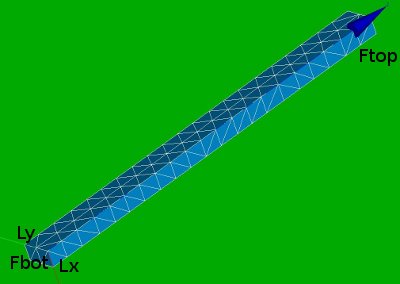
Fbot and Ftop are the bottom and top surfaces.
Lx and Ly are the edges along the x and y axes.

Non linear material behaviour

The non linear material behaviour is defined by the sigma epsilon curve. The CA commands for this relation are given by DEFI_FONCTION and DEFI_MATERIAU. The curve that has been used in this calculation is depicted below.

Sigma_eps = DEFI_FONCTION(NOM_PARA='EPSI',
                          VALE=(0.0016,	330,
                                0.0032,	350,
                                0.0064,	367,
                                0.0128,	387,
                                0.0200,	401,
                                0.0270,	410,
                                0.0400,	420,
                                0.0700,	437,
                                0.1000,	450,
                                0.1500,	473,
                                0.2000,	490,
                                0.3000,	510,),
                     INTERPOL='LIN',PROL_DROITE='LINEAIRE',PROL_GAUCHE='EXCLU',);

#define plastic behaviour of steel by Sigma_eps
steel=DEFI_MATERIAU(ELAS=_F(E=2.1e5,NU=0.27,),
                    TRACTION=_F(SIGM=Sigma_eps,),);

Note that the origin need not to be specified for the sigma epsilon in the DEFI_FONCTION.

The boundary conditions and the loads

For the boundary conditions we choose to fix:

• the bottom plane in axial (z) direction,
• the edge along the x axis in y direction and
• the edge along the y axis in x direction

LoadFix=AFFE_CHAR_MECA(MODELE=pmode,
                   FACE_IMPO=(_F(GROUP_MA='Fbot',DZ=0.0,),),
                   DDL_IMPO=(_F(GROUP_MA='Lx',DY=0.0),
                             _F(GROUP_MA='Ly',DX=0.0),),);
                   

For the load we apply an axial force on the top plane. The force is gradually increased to its maximum value, kept constant and reduced to zero again. This is performed by the multiplification function ramp in the load command.

# LoadPres will vary in the nonlinear calculation determined by the 'time' and  'ramp' function
# number of 'time' steps tsteps
# ramp increases during:
# 1.2 s: from 0.0 to 1.0, 
# 0.1 s: constant at 1.0
# 0.7 s: from 1.0 down to 0.3
dt = 0.10
t0 = 0.00
t1 = 1.20
t2 = t1+dt
t3 = 2.00
tsteps = int(t3*10)
disp = 0.0750
LoadPres=AFFE_CHAR_MECA(MODELE=pmode,
                   FACE_IMPO=(_F(GROUP_MA='Ftop',DZ=disp,),),);

ramp=DEFI_FONCTION(NOM_PARA='INST',
                  VALE=(t0,0.00,
                        t1,1.00,
                        t2,1.00,
                        t3,0.30,),
                  INFO=2,TITRE='ramp',);

time=DEFI_LIST_REEL(DEBUT=0.0,
                   INTERVALLE=_F(JUSQU_A=t3,NOMBRE=tsteps,),
                   INFO=2,TITRE='time',);

deflist = DEFI_LIST_INST(DEFI_LIST=_F(METHODE ='AUTO',
                                     LIST_INST = time,
                                     PAS_MINI = 0.0005),)

Presul=STAT_NON_LINE(MODELE=pmode,
                    CHAM_MATER=matprops,
                    EXCIT=(_F(CHARGE=LoadFix,),
                           _F(CHARGE=LoadPres,FONC_MULT=ramp,),),
                    COMP_INCR=_F(RELATION='VMIS_ISOT_TRAC',
                                 DEFORMATION='SIMO_MIEHE',
                                 TOUT='OUI',),
                    INCREMENT=_F(LIST_INST= deflist,), #time,
                    NEWTON=_F(REAC_INCR=1,
                              MATRICE='TANGENTE',
                              REAC_ITER=1,),
                    CONVERGENCE=_F(ITER_GLOB_MAXI=20,),
                    ARCHIVAGE=_F(PAS_ARCH=1,),);
                    

For comparison the linear calculation is applied as well:

LinRes=MECA_STATIQUE(MODELE=pmode,
                    CHAM_MATER=matprops,
                    #CARA_ELEM=shellch,
                    EXCIT=(_F(CHARGE=LoadFix,),
                           _F(CHARGE=LoadPres,),),);

The results of the linear calculation

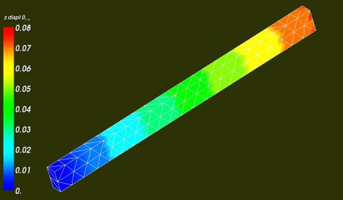
Axial displacement of the beam

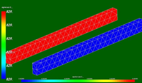
Elastic axial stresses sigma_zz (green beam, value 829 [MPa]) and strains eps_zz (blue beam, 3.95 [mm/m])

Theoretical verification: length of the beam: 19 mm cross section: 0.8*1.5 = 1.2 mm2 young's module: E = 2.1e5 MPa In the linear case, this yields a stress sigma and strain epsilon:

epsilon e_zz = dz/Lz = 0.075/19 = 0.00395 ~ 0.004 [-]

sigma = e_zz*E = 829 MPa

On the top 15 nodes the displacements and reaction forces are:

dz = 1.12500E+00 [mm] --> 0.075 mm at each node (that is correct)

Rz = -9.94737E+02 [N] --> pressure is Rz/A = -9.94737E+02/1.2 = 829 MPa (that is correct as well).