Difference between revisions of "Contrib:KeesWouters/solids/mooney-rivlin"
Keeswouters (Talk | contribs) m (→'''Initial stiffness''') |
Keeswouters (Talk | contribs) m (→''Geometry'') |
||
| Line 10: | Line 10: | ||
==''Geometry''== | ==''Geometry''== | ||
| − | This is really annoying. Once again a block. The dimensions are 2Xmax*2Ymax*Lz = 5x12x43 [mm3] (Xmax = 2.5, Ymax = 6, Lz = 43 [mm]). My only excuse is that it does show the behaviour of the material.<br/> | + | This is really annoying. Once again a block. The dimensions are 2Xmax*2Ymax*Lz = 5x12x43 [mm3] (Xmax = 2.5, Ymax = 6, Lz = 43 [mm]). My only excuse is that it does show the behaviour of the Mooney-Rivlin material very well.<br/> |
Four '''groups''' are defined on the block: | Four '''groups''' are defined on the block: | ||
* two areas, top and bottom areas, and | * two areas, top and bottom areas, and | ||
Revision as of 12:10, 1 October 2011
Contents
Material behaviour Mooney-Rivlin
preliminary. Have to check dimensions: stresses, pressures and stiffness coefficients: [Pa] or [MPa]
Simple block of Mooney-Rivlin material
september 2011 - Salome 6.3 - Code Aster VERSION DE DEVELOPPEMENT 11.00.10 - Ubuntu 11.04
This is a simple example of a block of Mooney-Rivlin material. As usual, the input and partly the output files can be found at the end of this contribution.
Errors are all mine.
Creative criticism welcome (of course I rather have positive than negative remarks).
Have fun.
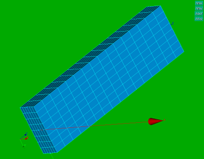
Geometry
This is really annoying. Once again a block. The dimensions are 2Xmax*2Ymax*Lz = 5x12x43 [mm3] (Xmax = 2.5, Ymax = 6, Lz = 43 [mm]). My only excuse is that it does show the behaviour of the Mooney-Rivlin material very well.
Four groups are defined on the block:
- two areas, top and bottom areas, and
- two node groups: centre node of the bottom plane and two nodes on the extreme positon of the y-axis.
The are used to define boundary conditions and pressure (load).
-
 :
: 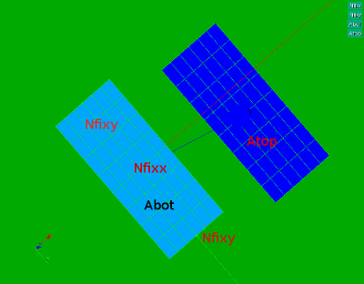


Loads and boundary conditions
A pressure of 6 [MPa] is applied to the top area Atop.
Note that to compare to analytic results with small strains, a pressure of 0.06 [MPa] has been used occasionally.
The boundary conditions are applied to the bottom area: all z displacements of the bottom area are restricted.
On node Nfixx the displacement in y direction is restricted.
On nodes Nfixy (two nodes on the extremes of the x axis) the displacement in x direction is restricted.
Code Aster commands
Material properties
The material properties are defined by Mooney-Rivlin.
This material behaviour is defined by a number of parameters (copied from JMB):
- C01 = 2.3456;
- C10 = 0.709;
- C20 = 0.0;
- NU = 0.499
- K = 6*(C10+C01)/(3*(1-2*NU))
and in Code Aster called by the hyper elastic material module:
rubber=DEFI_MATERIAU(ELAS_HYPER=_F(C10=C10,
                                   C01=C01,
                                   C20=C20,
                                   K=K,
                                   RHO=1000.0),);
The parameters Cxy are coefficients of the two invariants of the Strain energy function, see eg [wiki].
For small strains the shear modulus G can be expressed as twice the sum of C01 and C10: G = 2(C01 + C10). And Youngs modulus E is equal to E = 2G(1+nu). So we have E = 4(C01+C10)(1+nu). For incompressible material the possion ratio nu --> 0.5. Hence we use nearly incompressible material here using nu = 0.499. Note that the numerical value of the Youngs modulus is E = 18.3 [MPa] for the values above. Later on we will use this to verify the results.
The bulk modulus K is defined in terms of Youngs modulus en poisson ratio: K = E/(3*(1-2*nu)). For nu approaching to 0.5, K approaches to infinity, ie incompressible material.
Note that nu may not be set to 0.5 exactly (to machine precision). See also paragraph 3.7 (ELAS_HYPER) of the Opérateur DEFI_MATERIAU ([u4.43.01]
Commands
FORCE=AFFE_CHAR_MECA(MODELE=Mod3d,
                    PRES_REP=_F(GROUP_MA='Atop',
                                PRES=-6.000,),);
RAMPE=DEFI_FONCTION(NOM_PARA='INST',
               VALE=(0.0,0.0,
                     1.0,1.0,),
               INFO=2);
MatRub=AFFE_MATERIAU(MAILLAGE=Mesh,
                   MODELE=Mod3d,
                   AFFE=_F(TOUT='OUI',
                           MATER=rubber,),);
res=STAT_NON_LINE(MODELE=Mod3d,
                  CHAM_MATER=MatRub,
                  EXCIT=(_F(CHARGE=FORCE,FONC_MULT=RAMPE,),
                         _F(CHARGE=DEPL,),),
                  NEWTON=(_F(REAC_INCR=1,
                             MATRICE='TANGENTE',
                             REAC_ITER=1,)),
                  COMP_INCR=_F(RELATION='ELAS_HYPER',
                               DEFORMATION = 'GROT_GDEP',
                               TOUT='OUI',),
                  CONVERGENCE=(_F(ARRET='OUI',
                                   ITER_GLOB_MAXI=20)),
                  INCREMENT=_F(LIST_INST=LISTE,),);
Results
Displacements
We applying a pressure load of 6 [Pa] on the top area in 20 equal steps.
The picture below shows the overall displacements. The displacements are scaled to 1.

The picture below shows the displacements in x, y and z direction. The displacement in each direction are given. The maximum values are:
- dux = 0.63600 (both directions)
- duy = 1.52641 (both directions)
- duz = 43.441 (only positive direction)

Volume change
Since we put the poisson ratio nearly equal to 1/2 (nu ~ 0.5) we expect that the volume does not change. The undeformed state has a volume Vo = 2Xmax * 2Ymax * Lz = 2580 [mm3]. The deformed state has a volume of Vdef = 2(Xmax-dux)*2(Ymax-duy)*(Lz+duz) = 2583.1 [mm3], a change of 3.1 [mm3]. Taking into account the effect of the poisson ratio (nu=0.499) the volume change may be dV = Vo*eps*(1-2NU). Depending on the definition of eps this change of volume is 4.1 [mm3] (Note that maybe we have to take more digits of the displacements into account ...).
Initial stiffness
The small strain axial stiffness of the block is duz/Fz = duz/PA = Lz/AE. This yields for small strains duz = P*Lz/E. The pressure P is 6 [Pa], the length of the block in z direction is 43 [mm] and the Youngs modulus E = 6(C01+C10)*(1+nu) = 14.09 [mm].


This figure shows the displacement for an end-pressure-load of 0.06 [Pa] (also calculated using 20 steps). The displacement is 0.1417 [mm]. Scaled to 6 [Pa] the displacement is 14.17 [mm]. This is slightly more than the analytic value of 14.09 [mm].
The picture has been created by right clicking in the Object Browser of the PostPro module:
- PostPro
- <result_file.med>
- fields
- Resu1_depl --> Right Click
- in the pop up window (Evolution on Point - Parameters)
- select Field
- select Point (1535 - node in top plane)
- select Component (dz)
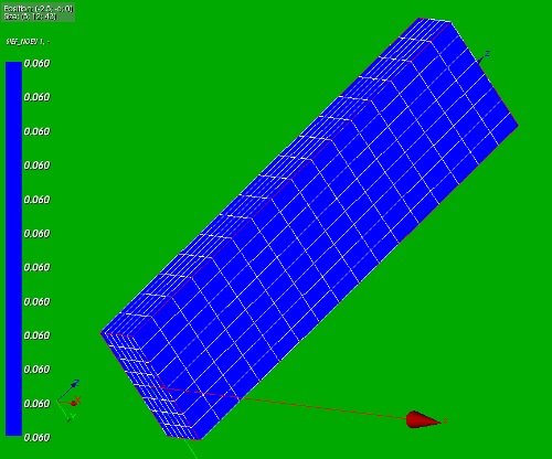
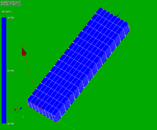
Stress and applied pressure
Again we have a look at the stresses (Szz) for small strains (applied pressure 0.06 [MPa]) and final stress (applied pressure 6 [MPa]. In the picture below the stresses are shown. Not very rewarding, all blue.
The small strain stress is 0.060 [MPa] (left/top picture). This corresponds with the applied pressure and initial cross section Ainitial = 5*12 = 60 [mm2]: Szz = F/A = PA/A = P = 0.06 [MPa].
The stress at large strain is 10.793 [MPa] (right/bottom picture). Now we have to do our home work. The applied pressure is 6 [Pa]. The cross section has been reduced to Astress = 4*(Xmax-dux)*(Ymax-duy) = 33.555 [mm2]. The initial cross section is Ainitial = 60 [mm2]. So the ultimate stress will be P*Ainitial/Astress = 6*60/33.555 = 10.793 [MPa]. Nice results.
Note that this includes that the applied pressure is not scaled to the real time area. The applied pressure is being translated to node forces initially and remain the same during the calculation.
-
 :
: 


Input files - download
Input files:
- Python script for defining the geometry and mesh. Load this file in Salome by File --> load script (cntrl T in the object browser), refresh (F5) after running.
- Save the mesh by:
- change to Mesh module
- right clicking in the object browser by right clicking on the mesh name Mblock; select Export to MED
- change mesh file name to Mblock.med (no need) and click save
- Save the mesh by:
- ASTK files (you need to edit the path to your requirements ...). To start Code Aster calculation press Run. Interactive enabled, Interactive-follow-up disabled, nodebug enabled.
- command file. Same remark as ASTK file.
Have fun.
Comments welcome.
Tested with CA version 11.00.10 and Salome 6.3.0.
groeten - Kees
Acknowledgement
I copied the material properties of JMB.