Difference between revisions of "Contrib:KeesWouters/plasticity"
Keeswouters (Talk | contribs) (→'''Boundary conditions and loads''') |
Keeswouters (Talk | contribs) (→'''Boundary conditions and loads''') |
||
| Line 61: | Line 61: | ||
=='''Boundary conditions and loads'''== | =='''Boundary conditions and loads'''== | ||
In Code Aster boundary conditions and loads are treated in the shame way. So no distinction need to be made between them. | In Code Aster boundary conditions and loads are treated in the shame way. So no distinction need to be made between them. | ||
| − | In the mesh we defined three groups for applying boundary conditions and loads: for fixed boundary conditions Pleft and Pright. In the command file they are united to one group | + | In the mesh we defined three groups for applying boundary conditions and loads: for fixed boundary conditions Pleft and Pright. In the command file they are united to one group Pfix by the command: |
pmesh=DEFI_GROUP(reuse =pmesh, | pmesh=DEFI_GROUP(reuse =pmesh, | ||
| Line 86: | Line 86: | ||
2.10,0.00,), | 2.10,0.00,), | ||
INFO=2,TITRE='ramp',); | INFO=2,TITRE='ramp',); | ||
| + | |||
| + | |||
| + | : [[image:Kw_time_ramp.jpg]] | ||
Revision as of 18:19, 12 August 2009
Contents
V shaped construction under plastic deformation
The V shaped is defined by an extrusion of a V shaped face.
-
 *
* 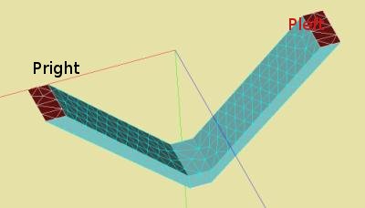


Three planes are defined in the geometry: Pleft and Pright for applyind boundary conditions (dx=dy=dz=0) and Pforce for defining a prescribed displacement in y direction.
The definition of the geometry as well as the meshing is given in the Python input file.
In the geometry module of Salome select File --> Load Script (or ctrl T) and thereafter the file: Media:kw_gm_vshape.zip.
General procedure of the calculation
The general procedure of the calculation is as follows:
- read the mesh
- apply the non linear material properties of the construction
- define the boundary conditions
- define the maximum load, in this case a maximum displacement at the plane Pforce
- define 'time' and 'load' increments:
- the time is defined from 0.0 to 2.1 and stepsize 0.1 s, yielding 21 points.
- The load multiplication factor is defined by ramping from 0.0 to 1.0 during the first 1 s,
- then keep it constant at 1.0 for 0.1 s and
- decreasing from 1.0 to 0.0 in the last second.
- perform the analysis
- define results in a med-file for Salome, in this case, displacements, vonMises and plastic stresses
- print results in a file, notably the displacements of the plane Pforce and its corresponding forces.

In the figure the results of four load cycles are given: the maximum displacement of each calculation is 0.080, 0.085, 0.095 and 0.100 mm. The plastic deformation at a load free construction after the load cycle is roughly 0.005, 0.009, 0.018 and 0.022 mm.
Each dot in the curves indicate a output point of the calculation. In most case 21 points are given, these have been defined in the 'time' increment function.
Non linear material properties
The linear material behaviour of steel is defined by the Young's modulus E = 210 GPa.

The plastic material behaviour is defined by TRACTTION and a table of (eps_i - sigma_i), as indicated in the figure. In the keyword DEFI_MATERIAU apart from Young's modulus and poisson ratio, now TRACTION is given for the non linear (eps-sigma) relation. The command AFFE_MATERIAU assigns the material to the complete mesh.
#Material properties
Traction=DEFI_FONCTION(NOM_PARA='EPSI',
                       VALE=(1.6e-3,300.0,
                             2.0e-2,400.0,
                             1.0e-1,450.0,
                             1.5e-1,473.0,
                             2.0e-1,500.0,
                             3.0e-1,550.0,),
                       INTERPOL='LIN',
                       PROL_DROITE='LINEAIRE',
                       PROL_GAUCHE='EXCLU',);
#define plastic behaviour of steel by Traction
steel=DEFI_MATERIAU(ELAS=_F(E=2.1e5,NU=0.27,),
                    TRACTION=_F(SIGM=Traction,),);
#assign material steel to the whole construction
matprops=AFFE_MATERIAU(MAILLAGE=pmesh,AFFE=_F(TOUT='OUI',MATER=steel,),);
Boundary conditions and loads
In Code Aster boundary conditions and loads are treated in the shame way. So no distinction need to be made between them. In the mesh we defined three groups for applying boundary conditions and loads: for fixed boundary conditions Pleft and Pright. In the command file they are united to one group Pfix by the command:
pmesh=DEFI_GROUP(reuse =pmesh,
                   MAILLAGE=pmesh,
                   CREA_GROUP_MA=(_F(NOM='Pfix',UNION= ('Pleft','Pright',),),),);
Of course, this could have been done in Salome just as well.
The boundary condition itself are given by:
LoadFix=AFFE_CHAR_MECA(MODELE=pmode,
                   FACE_IMPO=(_F(GROUP_MA='Pfix',
                                 DX=0.0,DY=0.0,DZ=0.0,),),);
The load will be applied in steps defined by a 'time' function and multiplification factor on the load.
tsteps = 21
time=DEFI_LIST_REEL(DEBUT=0.0,
                   INTERVALLE=_F(JUSQU_A=2.1,NOMBRE=tsteps,),
                   INFO=2,TITRE='time',);
ramp=DEFI_FONCTION(NOM_PARA='INST',
                  VALE=(0.00,0.00,
                        1.00,1.00,
                        1.10,1.00,
                        2.10,0.00,),
                  INFO=2,TITRE='ramp',);
