Difference between revisions of "Contrib:KeesWouters/prestressmodal"
Keeswouters (Talk | contribs) m (→'''The mesh of the cylinder''') |
Keeswouters (Talk | contribs) m (→'''The mesh of the cylinder''') |
||
| Line 36: | Line 36: | ||
==='''The mesh of the cylinder'''=== | ==='''The mesh of the cylinder'''=== | ||
| − | The mesh is defined in a | + | The mesh is defined in a Python script. It is generated by NetGen 1D_2D. By allowing quadrangles, a regular mesh with only this type of elements occur. Further options are: maxsize is 0.075, optimise, fineness is 3 and use second order, that is needed for coque_3d elements. Note the these quadratic quadrangles (quad8) need to be adapted to quad9 elements to be compatible with coque_3d elements in the command file. |
The names of the axial ends of the circumference and shell area are denoted by ''Cbot, Ctop and Surfin''. | The names of the axial ends of the circumference and shell area are denoted by ''Cbot, Ctop and Surfin''. | ||
Revision as of 10:05, 20 October 2009
Contents
Modal analysis of an axial loaded cylinder
[under construction .... not finished yet .... but maybe enough to be useful]
To start with, this contribution mainly focuses on the use of Salome and Code Aster, not on the results and the mechanical justifications of the code that has been used. So no guarantee that the results will be correct up to the fifth decimal place, which they are not. I do hope though that this information is useful. For me it has been, because I had to think about some commands and look through the documentation and learn from that. In case of mistakes, errors or remarks, please notify me, or better, you are invited to correct or edit them yourself. Enjoy.
As usual, the files that define the geometry, mesh and command files can be found at the end of this contribution.
Defining the mechanical properties of the cylinder
Geometry of the cylinder

The model is constructed by extrusion cq piping from a circle with diameter 4 mm. The extrusion is defined along a path along the z axis, defined by six points *), total length of the curve is 5 mm. The main commands of the python script are:
- define points:
- pz1 = geompy.MakeVertex(0.00, 0, 1)
- ....
- pz5 = geompy.MakeVertex(0.00, 0, 5)
- define circle: Circle = geompy.MakeCircle(centre, vector, radius)
- define path: Curve = geompy.MakePolyline([null, pz1, pz2, pz3, pz4, pz5 ])
- define cylinder: Pipe = geompy.MakePipe(Circle, Curve)
*) I used six points to do some experiments with the Pipe command. Of course, here is not necessary to use six points.
For applying boundary conditions and loads and use the shell elements later in the command file of Code Aster, we define the top and bottom circumference of the cylinder and the cylinder area:
- Surfin = geompy.CreateGroup(Pipe, geompy.ShapeType["FACE"])
- geompy.UnionIDs(Surfin, [25, 20, 15, 10, 3])
- Pipe = geompy.GetMainShape(Surfin)
- Ctop = geompy.CreateGroup(Pipe, geompy.ShapeType["EDGE"])
- geompy.UnionIDs(Ctop, [29])
- Pipe = geompy.GetMainShape(Ctop)
- Cbot = geompy.CreateGroup(Pipe, geompy.ShapeType["EDGE"])
- geompy.UnionIDs(Cbot, [8])
- Pipe = geompy.GetMainShape(Cbot)
The mesh of the cylinder
The mesh is defined in a Python script. It is generated by NetGen 1D_2D. By allowing quadrangles, a regular mesh with only this type of elements occur. Further options are: maxsize is 0.075, optimise, fineness is 3 and use second order, that is needed for coque_3d elements. Note the these quadratic quadrangles (quad8) need to be adapted to quad9 elements to be compatible with coque_3d elements in the command file.
The names of the axial ends of the circumference and shell area are denoted by Cbot, Ctop and Surfin.
The load and boundary conditions of the cylinder
The load and boundary conditions are defined in the Code Aster command file. The boundary conditions are at Cbot and Ctop:
- Cbot
- restrict displacements and rotations dx=dy=dz=drx=dry=drz=0 -->
- DDL_IMPO=(_F(GROUP_MA=('Cbot'),DX=0.0,DY=0.0,DZ=0.0,DRX=0.0,...),...
- Ctop
- restrict displacements and rotations dx=dy=drx=dry=drz=0 except dz -->
- DDL_IMPO=(...._F(GROUP_MA=('Ctop'),DX=0.0,DY=0.0,DRX=0.0,...),...
The load on the construction is an axial line force, total force is 7399.515 N -->
- dcyl = 4.00 # diameter of cylinder
- pie = math.pi
- Lcyl = pie*dcyl # circumference of the cylinder
- Fax = 7399.515
- Fclamp=AFFE_CHAR_MECA(...,FORCE_ARETE=_F(GROUP_MA='Ctop',FZ=+Fax/Lcyl,),);
Material properties of the beam
The beam consists of steel.
- steel=DEFI_MATERIAU(ELAS=_F(E=2.100e5,NU=0.28,RHO=0.007850),);
General procedure during the solution process
We will compare the modal behaviour of the unloaded and loaded cylinder. For the unloaded cylinder the standard modal analysis will be performed:
- determine stiffness matrix Smech and
- determine mass matrix Mmass
- carry out a modal analysis (Smech + lambda*Mmass)x = 0
For the pre stressed cylinder a modified modal analysis will be performed. The stiffness matrix is now given by the sum of the element stiffness matrix and geometrical stiffness matrix: Stiff = [Smech + Sgeom]:
- determine stiffness matrix Smech
- determine geometrical stiffness matrix Sgeom
- determine mass matrix Mmass
- carry out a modal analysis ([Smech + Sgeom] + lambda*Mmass)x = 0
Determining the geometrical stiffness matrix is exactly the same as in a buckling analysis. Details for the calculating the geometrical stiffness matrix can be found here: buckling analysis.
Modal analysis of the unloaded structure
Commands for modal analysis of the unloaded structure
The element stiffness matrix can be calculated by the following commands
- optional: perform static analysis [MECA_STATIQUE] *)
- determine stiffness matrix Smech [CALC_MATR_ELEM]
- determine mass matrix Mmass [CALC_MATR_ELEM]
*) Maybe used for testing the results, eg the boundary conditions and the load, the static analysis can be carried out. Though it is not really needed here.
Then, for the eigenvector calculation, the stiffness and mass matrices need to be correctly ordered according to the dofs (ddl) of the system, so
- determine ordering nddl [NUME_DDL]
- determine ordered SAmech [ASSE_MATRICE] and
- determine ordered SAmass [ASSE_MATRICE]
- perform eigenvalue analysis on SAmech and SAmass [MODE_ITER_SIMULT]
- project the results [PROJ_CHAMP] suitable for post processing in Salome (coque_3d ie quad9 --> quad8)
# for testing only
result=MECA_STATIQUE(MODELE=modelc,CHAM_MATER=matprops,
                    CARA_ELEM=shellch,EXCIT=_F(CHARGE=clamp,),);
# determine stiffness matrix of the structure and DDL vector
Smech = CALC_MATR_ELEM(OPTION = 'RIGI_MECA',
                                 MODELE = modelc,
                                 CARA_ELEM=shellch,
                                 CHARGE = clamp,
                                 CHAM_MATER = matprops,);
Mmass = CALC_MATR_ELEM(OPTION = 'MASS_MECA',
                                 MODELE = modelc,
                                 CHAM_MATER = matprops,
                                 CARA_ELEM = shellch,
                                 CHARGE = clamp,);
nddl   = NUME_DDL(MATR_RIGI=Smech);
SAmech = ASSE_MATRICE(NUME_DDL=nddl,MATR_ELEM=Smech,);
MAmass = ASSE_MATRICE(NUME_DDL=nddl,MATR_ELEM=Mmass,);
Rmodes=MODE_ITER_SIMULT(MATR_A=SAmech,
                        MATR_B=MAmass,
                        TYPE_RESU='DYNAMIQUE',
                        METHODE='SORENSEN',
                        CALC_FREQ=_F(OPTION='PLUS_PETITE',NMAX_FREQ=6,),);
SALmodes=PROJ_CHAMP(RESULTAT=Rmodes,
                    MODELE_1=modelc,
                    MODELE_2=modinit,);
IMPR_RESU(FORMAT='MED',UNITE=21,
          RESU=_F(MAILLAGE=meshinit,
          RESULTAT=SALmodes,
          NOM_CHAM='DEPL',),);
Numerical values of the eigenvalues of the unloaded structure
The eigenvalues can be obtained from the mess file. For the unloaded case, the six smallest eigenvalues are:
   NUMERO    FREQUENCE (HZ)    NORME D'ERREUR
        1      9.57306E+01       3.17056E-11
        2      9.57306E+01       3.14144E-11
        3      1.13379E+02       2.33041E-11
        4      1.13379E+02       2.30014E-11
        5      1.22476E+02       2.36309E-11
        6      1.22476E+02       1.96973E-11
NORME D'ERREUR MOYENNE:  0.25459E-10
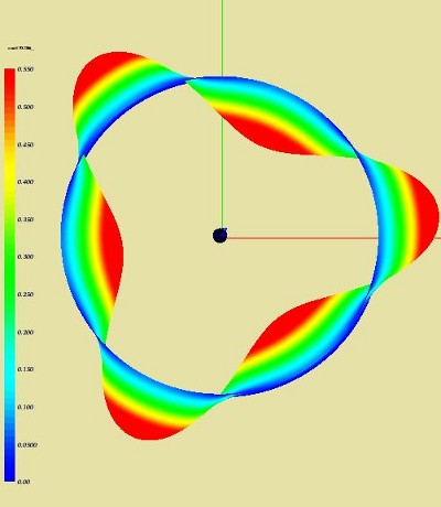
The first modal shape of the unloaded structure
The picture below denote the first modal shape at 96 Hz at different view points.
-
 *
* 


Modal analysis of the structure under prestress
Commands for modal analysis of the structure under prestress
The element stiffness matrix can be calculated by the following commands
- perform static analysis [MECA_STATIQUE], now needed to determine the stresses in the construction,
- determine the stresses [CREA_CHAMP] calculated in the static analysis,
- determine stiffness matrix Smech [CALC_MATR_ELEM],
- determine geometrical stiffness matrix Smech [CALC_MATR_ELEM], based on the stresses from the static analysis and
- determine mass matrix Mmass [CALC_MATR_ELEM]
Then, for the eigenvector calculation, the stiffness and mass matrices need to be correctly sorted according to the dofs (ddl) of the system, so
- determine ordering nddl [NUME_DDL],
- determine ordered SAmech [ASSE_MATRICE],
- determine ordered SAgeom [ASSE_MATRICE] and
- determine ordered SAmass [ASSE_MATRICE]
- perform eigenvalue analysis on SAmech and SAmass [MODE_ITER_SIMULT]
- project the results [PROJ_CHAMP] suitable for post processing in Salome (coque_3d --> quad8)
result=MECA_STATIQUE(MODELE=modelc,
                    CHAM_MATER=matprops,
                    CARA_ELEM=shellch,
                    EXCIT=_F(CHARGE=clamp,),);
Fsigma = CREA_CHAMP(OPERATION='EXTR',
                  TYPE_CHAM='ELGA_SIEF_R',
                  RESULTAT=result,
                  NUME_ORDRE=1,
                  NOM_CHAM='SIEF_ELGA_DEPL',);
# determine stiffness matrix of the structure and DDL vector
Smech = CALC_MATR_ELEM(OPTION = 'RIGI_MECA',
                                MODELE = modelc,
                                CARA_ELEM=shellch,
                                CHARGE = clamp,
                                CHAM_MATER = matprops,);
Sgeom = CALC_MATR_ELEM(OPTION='RIGI_GEOM',
                      MODELE=modelc,
                      CARA_ELEM=shellch,
                      SIEF_ELGA=Fsigma,);
Mmass = CALC_MATR_ELEM(OPTION = 'MASS_MECA',
                                MODELE = modelc,
                                CHAM_MATER = matprops,
                                CARA_ELEM = shellch,
                                CHARGE = clamp,);
nddl   = NUME_DDL(MATR_RIGI=Smech);
SAmech = ASSE_MATRICE(NUME_DDL=nddl,MATR_ELEM=Smech,);
SAgeom = ASSE_MATRICE(NUME_DDL=nddl,MATR_ELEM=Sgeom,);
MAmass = ASSE_MATRICE(NUME_DDL=nddl,MATR_ELEM=Mmass,);
Stotal = COMB_MATR_ASSE(COMB_R=(_F(MATR_ASSE=SAmech,COEF_R=1.0,),
                               _F(MATR_ASSE=SAgeom,COEF_R=1.0,),),);
Rmodes=MODE_ITER_SIMULT(MATR_A=Stotal,
                       MATR_B=MAmass,
                       TYPE_RESU='DYNAMIQUE',
                       METHODE='SORENSEN',
                       CALC_FREQ=_F(OPTION='PLUS_PETITE',NMAX_FREQ=6,),);
SALmodes=PROJ_CHAMP(RESULTAT=Rmodes,
                   MODELE_1=modelc,
                   MODELE_2=modinit,);
IMPR_RESU(FORMAT='MED',UNITE=21,
         RESU=_F(MAILLAGE=meshinit,
         RESULTAT=SALmodes,
         NOM_CHAM='DEPL',),);
Calculating matrices by MACRO_MATR_ASSE
The sorted stiffness and mass matrices have been determined by the two commands CALC_MATR_ELEM and ASSE_MATRICE. It is also possible to use a single command: MACRO_MATR_ASS.
Smech = CALC_MATR_ELEM(OPTION = 'RIGI_MECA',MODELE = modelc,CARA_ELEM = shellch,CHAM_MATER = matprops,CHARGE = clamp,);
Mmass = CALC_MATR_ELEM(OPTION = 'MASS_MECA',MODELE = modelc,CARA_ELEM = shellch,CHAM_MATER = matprops,CHARGE = clamp,);
Sgeom = CALC_MATR_ELEM(OPTION = 'RIGI_GEOM',MODELE = modelc,CARA_ELEM = shellch,SIEF_ELGA = Fsigma,);

nddl   = NUME_DDL(MATR_RIGI=Smech);
SAmech = ASSE_MATRICE(NUME_DDL=nddl,MATR_ELEM=Smech,);
SAgeom = ASSE_MATRICE(NUME_DDL=nddl,MATR_ELEM=Sgeom,);
MAmass = ASSE_MATRICE(NUME_DDL=nddl,MATR_ELEM=Mmass,);
In stead you can use the MACRO_MATR_ASSE command:
MACRO_MATR_ASSE(MODELE=modelc,CHAM_MATER=matprops,CARA_ELEM=shellch,CHARGE=clamp,
               NUME_DDL=CO('nddl'),  # define 'nddl' here
               MATR_ASSE=(_F(MATRICE=CO('SAmech'),OPTION='RIGI_MECA',),
                          _F(MATRICE=CO('MAmass'),OPTION='MASS_MECA',),),);
MACRO_MATR_ASSE(MODELE=modelc,
               #CHAM_MATER=matprops,
               CARA_ELEM=shellch,
               CHARGE=clamp,
               NUME_DDL=nddl,     # nddl already defined prevously
               MATR_ASSE=(_F(MATRICE=CO('SAgeom'),OPTION='RIGI_GEOM',SIEF_ELGA=Fsigma,),),);
Remark:
- because the geometrical stiffnessmatrix does not require and does not accept the CHAM_MATER option, the calculation of the geometrical stiffness matrix has been seperated from the stiffness and mass matrices.
- the definition the nddl can only occur once, so in the first MACRO_MATR_ASSE command use NUME_DDL=CO('nddl') to define and calculated nddl. Then in the second command it can be used directly as NUME_DDL=nddl.
Numerical values of the eigenvalues of structure under prestress
The eigenvalues can be obtained from the mess file. For the unloaded case, the six smallest eigenvalues are:
   NUMERO    FREQUENCE (HZ)    NORME D'ERREUR
        1      1.30828E+02       1.63671E-11
        2      1.30828E+02       1.71866E-11
        3      1.44320E+02       1.49786E-11
        4      1.44320E+02       1.45535E-11
        5      1.51135E+02       1.51974E-11
        6      1.51135E+02       1.48339E-11
NORME D'ERREUR MOYENNE:  0.15520E-10
And compared to the non loaded structure, we have
       loaded  no load difference
	[Hz]	 [Hz]	    [%]
1	130.8	  95.7	    37
2	130.8	  95.7	    37
3	144.3	 113.4	    27
4	144.3	 113.4	    27
5	151.1	 122.5	    23
6	151.1	 122.5	    23
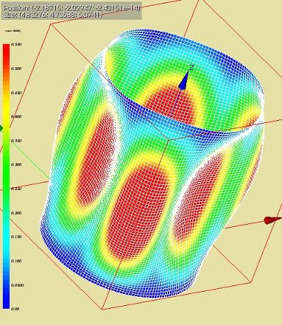
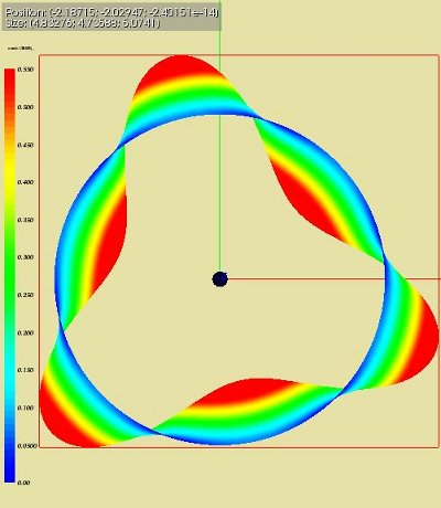
The first modal shape of the loaded structure
The picture below denote the first modal shape at 131 Hz from different view points.
-
 *
* 


Write the total mass of the construction
Using the MASS_INER command, the total mass of the construction can be written to a file (here on UNITe 26, defined in ASTK as npcyl.txt, download at the end)
masshell=POST_ELEM(MASS_INER=_F(GROUP_MA='Surfin',ORIG_INER=(0.0, 0.0, 0.0),),
                   MODELE=modelc,
                   CHAM_MATER=matprops,
                   CARA_ELEM=shellch,);
IMPR_TABLE(TABLE=masshell,UNITE=26,NOM_PARA='MASSE',);
The content of the results file is:
.....
#ASTER  9.04.00 CONCEPT masshell CALCULE LE 03/09/2009 A 17:53:48 DE TYPE
#TABLE_SDASTER
MASSE
 4.93230E-02
This agrees with the mass calculated by:
- mass = rho * Volume = rho * pi*Dcyl*Hcyl*th = 0.00785*pi*4*5*0.1 = 0.0493 kg.
Buckling analysis
The prestress in the construction is determined such that the buckling load is -1, eg. the both the element stiffness and the geometrical stiffness have roughly the same order of magnitude. The command is as follows:
# multiply results by -1 or reverse force, since we solve
# A*x = lamdba*B*x iso (A+mu*B)x=0
Rbuckle = MODE_ITER_SIMULT(INFO=1,
                         MATR_A  = SAmech,
                         MATR_B  = SAgeom,
                         METHODE = 'SORENSEN',
                         PREC_SOREN=2e-16,
                         NMAX_ITER_SOREN=250,
                         TYPE_RESU='MODE_FLAMB',
                         CALC_FREQ=_F(OPTION='PLUS_PETITE',NMAX_FREQ=4,),);
IMPR_RESU(FORMAT='MED',
         UNITE=21,
         RESU=_F(MAILLAGE=meshinit,
                 RESULTAT=Rbuckle,
                 NOM_CHAM='DEPL',),);
and the corresponding four lowest buckling loads are, see mess file:
   NUMERO    CHARGE CRITIQUE    NORME D'ERREUR
        1      9.86304E-01       6.80828E-12
        2      9.86305E-01       6.84256E-12
        3      9.99999E-01       5.58740E-12
        4      1.00000E+00       5.56880E-12
NORME D'ERREUR MOYENNE:  0.62018E-11
The load at number 4 corresponds to a total axial force of Fax = 7399.515 N. The corresponding bluckling mode is given below.
Note:
- that we applied an axial pulling force, and again, the lowest buckling load at 4 need to be multiplied by -1 because of the implementation of the eigenvalue analysis in Code Aster.
- that the highest value of charge-critique corresponds to the lowest critical load.
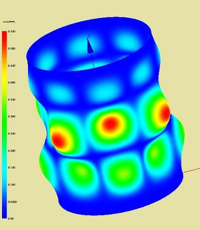
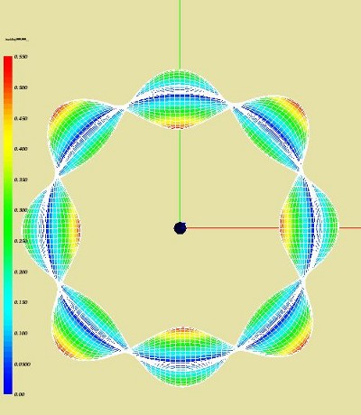
The buckling mode of the loaded structure
The picture below denote the lowest buckling mode for an axial load of 7399.515 N at different view points.
-
 *
* 


The displacement according to Code Aster at the outer edge Ctop of the cylinder is 0.1387 mm for the given axial load. The analytical displacement is
- dL = F*L/(E*A) = 0.1402:
- F = 7399.515 N
- L = 5.00 mm (height of the cylinder)
- E = 2.1e5 MPa
- A = pi*D*th = 1.2566 mm2, D is diameter and th is thickness of the cylinder.
ASTK files
In the picture below the various input and output files of the calculation are given.

Download files
This zip contains the following files
- python geometry and mesh files (load in Salome by File --> Load script (cntrl T)) and right select refresh (F5) in the object browser). Export the med file in the mesh module under cylinder.med for further processing by Code-Aster, controlled by ASTK.
- command files for Code-Aster:
- - cyl_modal.comm, modal analysis of the unloaded structure
- - cyl_loaded.comm, modal analysis of the structure under pre stress, buckling also included
- astk file for file control by ASTK
- npcyl.txt, text file with nodal displacements and force on plane top and total mass of the structure, not very spectacular.
The result file buck2res.med can be viewed in the post processor module of Salome by File --> Import --> buck2res.med or cntrl I in the object browser.
that is all for now
september 2009
kees wouters